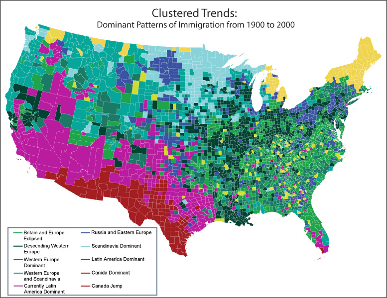
This cluster analysis shows trends of immigrant proportion – not immigrant percent. Therefore if, in 2000, 60% of the residents in County A are immigrants, and 10% of the residents in County B are immigrants, but both Counties’ immigrants are 80% Latin American and 20% Russian, these two counties will have exactly the same trend point in 2000.
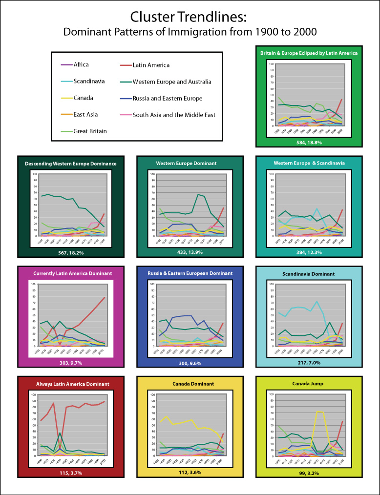
The trend chart symbols show a variation of immigration trends across the US, which may be placed into three categories: Latin American dominant (red or pink), Canada dominant (yellow-ish), or European Dominant (greenish-blueish). Each trend chart denotes, at bottom, the number and percent of counties represented by that particular trend.
It is interesting that the counties closest to the Mexico border have had consistently high numbers of Latin American immigrants throughout the century, while the counties slightly above the border have seen the most dramatic increase in Latin American immigrants. Both of the Latin America trend charts display an impossible dip of Latin American immigrants in 1930, along with an odd spike in other immigrant groups. This is probably a simple data error, though it is perhaps possible that, due to political pressures in 1930, Latin American immigrants uniformly chose to mark a European country as their country of origin. This would be a fascinating social phenomenon, but unlikely to have occurred so uniformly.
The trend labeled “Canada Dominant” seems logically placed on the map, but the trend labeled “Canada Jump” seems less logical. There seems to be no obvious reason behind a massive emigration of Canadians to these counties in 1960, especially as it corresponds with a dip in other immigrant group numbers. As this trend represents only 3.2% of all counties, it is almost certainly an error.
The European trend charts all show a high number of Western European immigrants, declining over the years and meeting a rising number of Latin American immigrants in the last third of the century. Within this group, however, we see that certain areas of the US drew particular types of Europeans – Scandinavians, British, Eastern Europeans and Russians, etc. Interestingly, the trend-lines show us that, over the years, the dominant European group of the cluster declines, while the other European groups stay mostly constant in number. This appears to illustrate a decline in the level of geographic segregation between European immigrants over time, perhaps due to a greater socio-economic differentiation between national identities in the past.
Interestingly, every cluster besides the two Latin America Dominant clusters shows a very similar proportion of Latin American immigrants in 2000 – all about 35%. This certainly does not represent the true variation between county proportions of Latin American immigrants. However, as Latin American immigrant numbers are quite small and recent compared to the longer history of European presence, current Latin American proportions are not the driving factor behind cluster formation. Therefore, any variation in current Latin American proportion that might occur within clusters is hidden by the averaging of county trends. In a couple decades, however, Latin American immigration might indeed be the driving factor behind differentiation of clusters in any similar cluster analysis.